Estimating SGD NEER in Python

Singapore’s monetary policy is operated by targeting its Nominal Effective Exchange Rate (NEER). The Monetary Authority of Singapore (MAS) follows a policy of an appreciating NEER to keep imported inflation in check and stabilize the competitiveness of Singapore’s exports.

Dubbed as the Band Basket and Crawl (BBC) policy, MAS lets the NEER fluctuate within a certain range (the Band) around a midpoint determined by the central bank. The NEER itself is calculated as a weighted average of the FX rates of Singapore’s major trading partners (the Basket). Finally, the midpoint is allowed to appreciate at a pre-determined pace (the Crawl) judged appropriate by MAS.

Given its structure and construction, the pace of NEER appreciation can be controlled by changing the mid-point of the band, changing (or even eliminating) the crawl or by widening/narrowing the band. A lower mid-point, a slower crawl and a narrower band decrease the pace of NEER appreciation. Conversely a higher mid-point, a faster crawl and a wider band increase the pace of NEER appreciation. 

The MAS releases a weekly average of the NEER level. However, it neither discloses the width of the band nor the constituents of the NEER basket nor the pace of crawl. Analysts rely on the MAS’s monetary policy statements to glean information about the dynamic trends in NEER and tweak their own NEER estimates so as to closely track the official NEER.

This article shows how to estimate the SGD NEER using econometric analysis in Python using Pandas, SciPy and other relevant libraries.

Preparing the data

A good approach is to select the most recent period of stable policy which begins when the MAS re-centered the NEER mid-point on 14 October 2022 and continues till now. This gives us more than 100 data points.

The data series required for our NEER estimation are – the official NEER and the SGD cross rates viz a viz Singapore’s trading partners. I downloaded them from the MAS database into an excel file.

Before we turn to estimation, we need to rescale the data by indexing it to 21 October 2022 (the first datapoint since the policy change) as the base date.

Next we calculate weekly FX returns by taking the difference of the natural logs for all the data series. This gives us the continuous compounding returns and makes returns additive over time. Finally, we multiply the FX returns of the cross rates with minus one. This is to convert the FX returns to reflect SGD as the base currency.

# Importing the relevant libraries
import pandas as pd
import numpy as np

# Importing data from excel into pandas dataframe called df
df=pd.read_excel("C:/Users/Macrologue/mas.xlsx")
df.info()
df.describe()

# Setting the Date column to be the index of the dataframe
df['Date'] = pd.to_datetime(df['Date'])
df.set_index('Date', inplace=True)

# Setting 21 Oct 2022 as the base date
base_date = '2022-10-21'
indexed_df = df / df.loc[base_date]
indexed_df = indexed_df * 100

# Calculating log returns and dropping the rows with missing data
log_returns = indexed_df.apply(lambda x: np.log(x / x.shift(1)))
df = log_returns.dropna()

# Multiplying cross rates with minus one to convert FX returns into SGD as base currency

df1= df[['EUR','GBP','USD','AUD','CAD','CNY','HKD','INR','IDR','JPY','KRW','MYR','TWD','NZD','PHP','QAR','SAR','CHF','THB','AED','VND'
]]*-1
df1['NEER']=df['NEER']

Constrained Optimization

We now estimate how the NEER is influenced by fluctuations in the cross rates of Singapore’s trading partners. This is done by fitting a regression equation with NEER returns as the dependent variable and returns on the cross rates as independent variables.

The estimated betas on the cross rates would be the weights of the relevant currencies in the NEER basket. Since we want our weights to sum to one we fit the regression equation with the added constraint that the estimated beta coefficients sum to one. This is achieved by using SciPy’s optimize function.

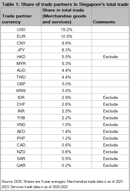
There are 21 trade partners, accounting for 83% of total trade, for which cross rates are available. See Table 1 on the right for the trade shares of individual countries.

We begin the optimization exercise with the full set of currencies and then narrow down the explanatory variables to achieve a closer fit to the MAS NEER as reflected by the mean square error (MSE). Note that USD linked currencies such as HKD are highly correlated with the USD and don’t really add any unique information to the dataset. So it makes sense to exclude them. This brings down our MSE from 0.12 to 0.07.

Next, we sequentially exclude the currencies with the lowest trade shares and work our way upwards till further improvements to MSE disappear. See Table 2 below for the MSE trend.

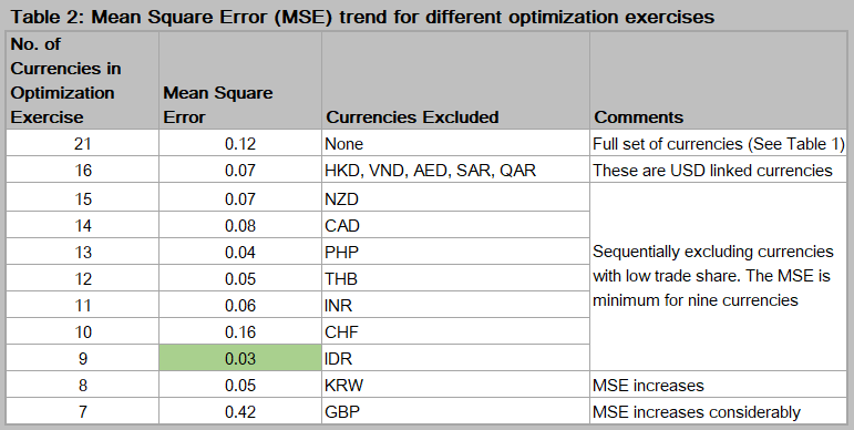
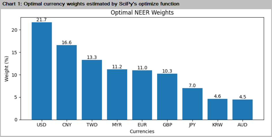
We find that the model works best with nine currencies (MSE equals 0.03) and further exclusions increase the MSE considerably. The optimized betas are the implied weights of the trade partner currencies in the NEER and are plotted in Chart 1.

import statsmodels.api as sm
from scipy.optimize import minimize

# Specifying the Dependent and Independent variables
Y = df1['NEER'].values
X = df1[['EUR','GBP','USD','AUD','CNY','JPY','KRW','MYR','TWD']].values


# Defining the objective function - Sum of Squared Residuals
def objective_function(betas):
    Estimated_Y = np.dot(X, betas)
    return np.sum((Y - Estimated_Y) ** 2)

# Defining the constraint - sum of betas equals 1
constraints = {
    'type': 'eq',
    'fun': lambda betas: np.sum(betas) - 1
}

# Specifying the initial guess for betas - use any numbers that sum to 1
initial_betas = np.full(9, 1/9)

# Minimize the objective function and calculating the estimated values
result = minimize(objective_function, initial_betas, constraints=constraints)

optimized_betas = result.x
df1['Estimated_Y'] = np.dot(X, optimized_betas)

# The estimated weights on individual currencies are simply the optimized_betas multiplied with 100
Weights = [x*100 for x in optimized_betas]

# Assigning the corresponding FX names to the Weights and sorting in descending order
Currency=['EUR','GBP','USD','AUD','CNY','JPY','KRW','MYR','TWD']

Currency_Weights_dict = dict(zip(Currency, Weights))

sorted_Currency_Weights = sorted(Currency_Weights_dict.items(), key=lambda item: item[1], reverse=True)

# Plotting the estimated Weights
import matplotlib.pyplot as plt
plt.figure(figsize=(8, 4))
bars=plt.bar([p[0] for p in sorted_Currency_Weights], [p[1] for p in sorted_Currency_Weights])

for bar in bars:
    yval = bar.get_height()
    plt.text(bar.get_x() + bar.get_width()/2, yval, round(yval, 1), ha='center', va='bottom')

plt.xlabel('Currency')
plt.ylabel('Weight (%)')
plt.title('Optimal NEER Weights')
plt.tight_layout()

plt.show()

The USD has the largest weight (21.7%) in the estimated NEER followed by CNY (16.6%).

We now plot the estimated NEER from our optimization exercise versus the official NEER in Chart 2.

# Calculating cumulative log returns for deriving the official NEER (NEERo) and estimated NEER (NEERe)
cumulative_log_returnsY = np.cumsum(df1['NEER'])
NEERo = 100 * np.exp(cumulative_log_returnsY)

cumulative_log_returnsYhat = np.cumsum(df1['Estimated_Y'])
NEERe = 100 * np.exp(cumulative_log_returnsYhat)

# Plotting offical vs. estimated NEER
plt.figure(figsize=(8, 4))
plt.plot(NEERo, label='Official NEER')
plt.plot(NEERe, label='Estimated NEER')
plt.title('NEER levels, 21 Oct 2022=100')
plt.legend()
plt.show()

The correlation between the official and estimated NEER stands at 0.991

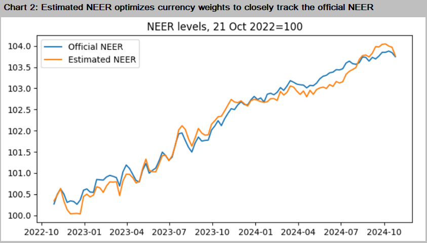
Given the tight correlation between the official and estimated NEER we can use the optimized betas to construct a proxy basket of a few currencies to take up short or long positions on the SGD NEER.